

August 6, 2004
Updated:Toy Example Demonstrating the Feasiblity of Grading an Anesthesiologist
|
This is an application of activity inference that we have been working on at Intel. The basic problem is to assign a grade to someone's performance of an activity based on observing an RFID sensor stream. In particular we would like to grade novice anesthesiologists in their performance of the intubation procedure. This article describes the technical approach that we are taking and some preliminary problems with toy examples. |
For this example we are going to assume that we are given a model of different ways of completing an activity as shown in Figure 1. Imagine that these are three different ways of drawing blood from a patient. At each step in the activity we observe something about the world. These observations are represented by letters. They could be RFID tags or many other types of sensor input. This model expresses the fact that in order to draw blood in one way (states 0->1->2->3->4) you must start the activity ("*"), then touch an "A", "B","C", and "D" in that order. Because we live in a fallen world, we occasionally don't see things that we ought to. So just because you don't see "ABCD" doesn't mean that you didn't draw blood using the first technique, but we'll assume that we can characterize the error with a false positive rate and a false negative rate. For this example I assumed that both of them are 25%. So 25% of the time, the things that I did touch I don't see and 25% of the time things that I didn't touch appear to be touched. This model is therefore a Hidden Markov Model. If we were to actually draw blood using the first technique, but, because of sensor errors, we saw the sequence "ABCH", we would want a system to infer a lower probability than "ABCD".
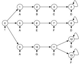 Figure 1
Now for the proposed scheme, in order to grade students, we are going to ask the student to perform the blood draw using the third technique such that the objects "AGCD" are touched when the procedure is done correctly. In this case the model is simple and the inference could be done exactly, but we have a particle filter implementation in our toolbox, so I'm going to hit this problem with that hammer. A particle filter gives approximate solutions. When I run the particle filter on the observation sequence "*AGCD" it reasons as follows:
| State\Observation | * | A | G | C | D |
| 0 | 1.000 | 0 | 0 | 0 | 0 |
| 1 | 0 | 0.337 | 0 | 0 | 0 |
| 2 | 0 | 0 | 0.055 | 0 | 0 |
| 3 | 0 | 0 | 0 | 0.058 | 0 |
| 4 | 0 | 0 | 0 | 0 | 0.101 |
| 5 | 0 | 0.324 | 0 | 0 | 0 |
| 6 | 0 | 0 | 0.053 | 0 | 0 |
| 7 | 0 | 0 | 0 | 0.003 | 0 |
| 8 | 0 | 0 | 0 | 0 | 0.005 |
| 9 | 0 | 0.339 | 0 | 0 | 0 |
| 10 | 0 | 0 | 0.891 | 0 | 0 |
| 11 | 0 | 0 | 0 | 0.937 | 0 |
| 12 | 0 | 0 | 0 | 0 | 0.838 |
| 13 | 0 | 0 | 0 | 0 | 0.054 |
| total | ~1.0 | ~1.0 | ~1.0 | ~1.0 | ~1.0 |
So the way that you can interpret these results are as follows. If the student was supposed to draw blood in the third way (with the D option on the tail) then the system is 84% sure that that is what they did. If the student was supposed to draw blood in the first way and generated the same sequence of observations, then the system is 10% sure that that is what the student did.
If the student had instead generated the sequence "*AGCF" then the system would have been 5% sure that they drew the blood in the third way (this scenario is not represented in the table).
Just for comparison if the student generated the sequence "*HHHH", by touching completely unrelated things, then the system would have been 16% sure that s/he drew blood in that way. That's a problem. We don't want "HHHH" to look more like drawing blood than "AGCF." It is a problem because we are forcing the model to explain the observations.
The trick here is that the probabilities are a result of normalizing the likelihoods during the runs. The likelihoods are of the form P(observation|state). As soon as you normalize the likelihoods, they are no longer relative to all other possible observations, they become relative to the possible states: P(state| observations). If we don't re-normalize the likelihoods we get the following likelihoods:
| State\Observation | * | A | G | C | D |
| 0 | 1000 | 0 | 0 | 0 | 0 |
| 1 | 0 | 337.0 | 0 | 0 | 0 |
| 2 | 0 | 0 | 21.0625 | 0 | 0 |
| 3 | 0 | 0 | 0 | 56.0 | 0 |
| 4 | 0 | 0 | 0 | 0 | 56.0 |
| 5 | 0 | 324.0 | 0 | 0 | 0 |
| 6 | 0 | 0 | 20.25 | 0 | 0 |
| 7 | 0 | 0 | 0 | 3.125 | 0 |
| 8 | 0 | 0 | 0 | 0 | 3.0 |
| 9 | 0 | 339.0 | 0 | 0 | 0 |
| 10 | 0 | 0 | 339.0 | 0 | 0 |
| 11 | 0 | 0 | 0 | 894.0 | 0 |
| 12 | 0 | 0 | 0 | 0 | 461.0 |
| 13 | 0 | 0 | 0 | 0 | 30.0 |
| total | 1000 | 1000 | 380.3125 | 953.125 | 550 |
So if you normalize the likelihoods in the final time step you get the same answer 461/(56.0+3.0+461.0+30.0) = 83.8% , but now we can compare the likelihood (or score if you prefer) that the model gives "*AGCD" in this case to the score it gives "*AGCF" and "*HHHH" (This alternative observation sequences are not shown in the table above.
| *AGCD | 461 |
| *AGCF | 28 |
| *HHHH | 10 |
Now this is much better because it shows that relative to the other possible observation sequences the scores make sense. This allows you to rank all the students in a class. If you wanted a probability score, you would have to try all possible observations and then normalize them to get P(observations|third blood draw).
So the remaining problem is that of assigning grades. If the best sequence that a user could generate gave a score of 461 and exchanging one object caused the score to drop to 28, then exchanging all four objects drops the score to 10. then it might be hard to pick a threshold of passing automatically.
Posted by djp3 at August 6, 2004 10:29 AM | TrackBack (0)